library(dplyr)
library(tidyr)
library(purrr)
library(ggplot2)
library(scales)
library(klaR)
library(cluster)Clustering Binary Data
R
Unsupervised Learning
An application of different unsupervised learning approaches to cluster simulated survey responses using R
In this post, I tackle the challenge to extract a small number of typical respondent profiles from a large scale survey with multiple yes-no questions. This type of setting corresponds to a classification problem without knowing the true labels of the observations – also known as unsupervised learning.
Technically speaking, we have a set of \(N\) observations \((x_1, x_2, ... , x_N)\) of a random \(p\)-vector \(X\) with joint density \(\text{Pr}(X)\). The goal of classification is to directly infer the properties of this probability density without the help of the correct answers (or degree-of-error) for each observation. In this note, we focus on cluster analysis that attempts to find convex regions of the \(X\)-space that contain modes of \(\text{Pr}(X)\). This approach aims to tell whether \(\text{Pr}(X)\) can be represented by a mixture of simpler densities representing distinct classes of observations.
Intuitively, we want to find clusters of the survey responses such that respondents within each cluster are more closely related to one another than respondents assigned to different clusters. There are many possible ways to achieve that, but we focus on the most popular and most approachable ones: \(K\)-means, \(K\)-modes, as well as agglomerative and divisive hierarchical clustering. As we see below, the 4 models yield quite different results for clustering binary data.
We use the following packages throughout this post. In particular, we use klaR and cluster for clustering algorithms that go beyond the stats package that is included with your R installation.1
Note that there will be an annoying namespace conflict between MASS::select() and dplyr::select()). We use the conflicted package to explicitly resolve these conflicts.
library(conflicted)

conflicts_prefer(
  dplyr::filter,
  dplyr::lag,
  dplyr::select
)
Creating sample data
Let us start by creating some sample data where we basically exactly know which kind of answer profiles are out there. Later, we evaluate the cluster models according to how well they are doing in uncovering the clusters and assigning respondents to clusters. We assume that there are 4 yes/no questions labeled q1, q2, q3 and q4. In addition, there are 3 different answer profiles where cluster 1 answers positively to the first question only, cluster 2 answers positively to question 2 and 3 and cluster 3 answers all questions positively. We also define the the number of respondents for each cluster.
centers <- tibble(
  cluster = factor(1:3),
  respondents = c(250, 500, 200),
  q1 = c(1, 0, 1),
  q2 = c(0, 1, 1),
  q3 = c(0, 1, 1),
  q4 = c(0, 0, 1)
)
Alternatively, we could think of the yes/no questions as medical records that indicate whether the subject has a certain pre-condition or not.
Since it should be a bit tricky for the clustering models to find the actual response profiles, let us add some noise in the form of respondents that deviate from their assigned cluster profile and shuffle all rows. We find out below how the cluster algorithms are able to deal with this noise.
set.seed(42)
labelled_respondents <- centers |>
  mutate(
    across(
      starts_with("q"),
      ~map2(respondents, .x, function(x, y) {
        rbinom(x, 1, max((y - 0.1), 0.1))
      }),
      .names = "{col}"
    )
  ) |>
  select(-respondents) |>
  unnest(cols = c(q1, q2, q3, q4)) |>
  sample_n(n())
The figure below visualizes the distribution of simulated question responses by cluster.
labelled_respondents |>
  pivot_longer(cols = -cluster,
               names_to = "question", values_to = "response") |>
  mutate(response = response == 1) |>
  ggplot(aes(x = response, y = question, color = cluster)) +
  geom_jitter() +
  theme_bw() +
  labs(x = "Response", y = "Question", color = "Cluster",
       title = "Visualization of simulated question responses by cluster")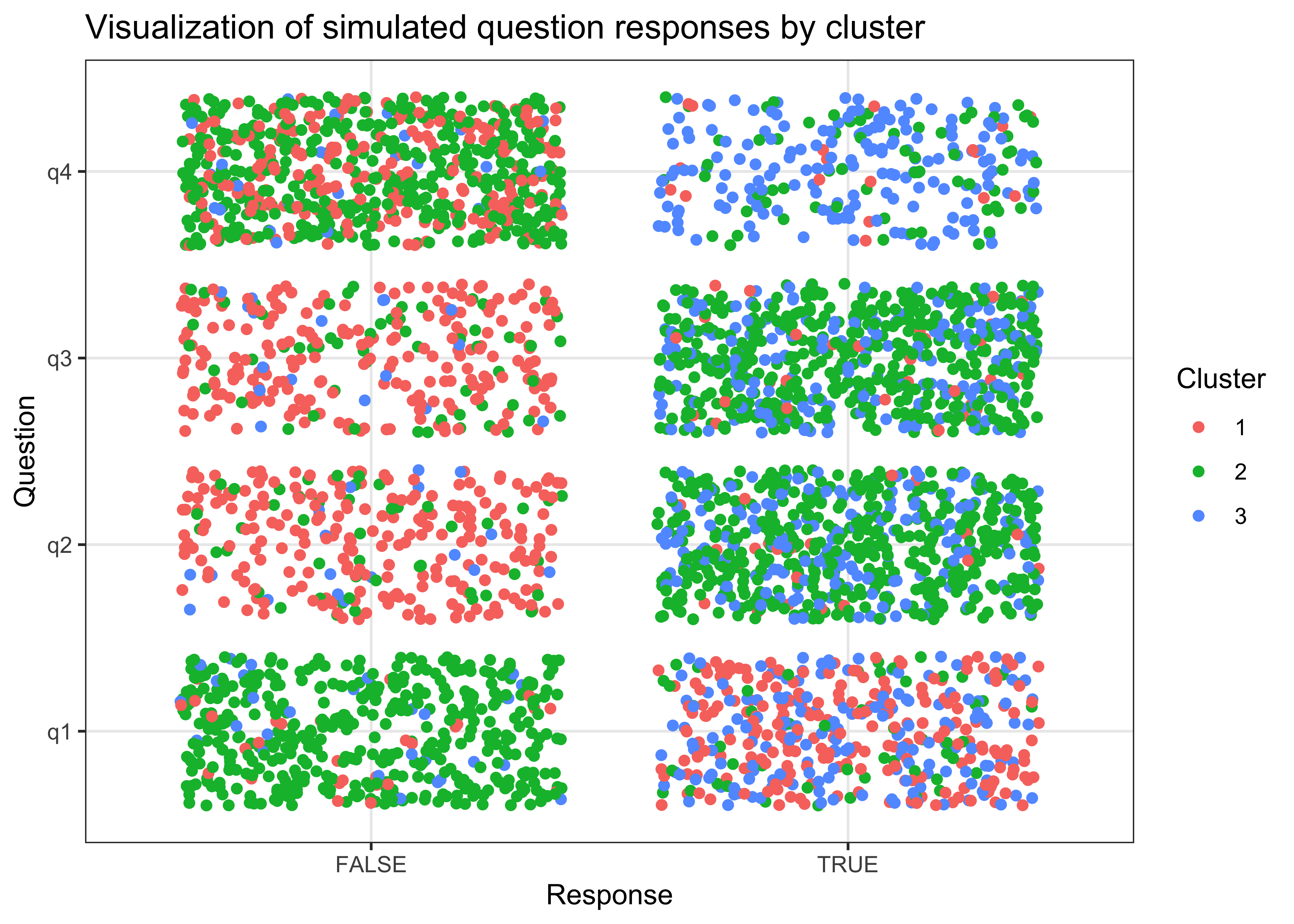
\(K\)-means clustering
The \(K\)-means algorithm is one of the most popular clustering methods (see also this tidymodels example). It is intended for situations in which all variables are of the quantitative type since it partitions all respondents into \(k\) groups such that the sum of squares from respondents to the assigned cluster centers are minimized. For binary data, the Euclidean distance reduces to counting the number of variables on which two cases disagree.
This leads to a problem (which is also described here) because of an arbitrary cluster assignment after cluster initialization. The first chosen clusters are still binary data and hence observations have integer distances from each of the centers. The corresponding ties are hard to overcome in any meaningful way. Afterwards, the algorithm computes means in clusters and revisits assignments. Nonetheless, \(K\)-means might produce informative results in a fast and easy to interpret way. We hence include it in this post for comparison.
To run the \(K\)-means algorithm, we first drop the cluster column.
respondents <- labelled_respondents |>
  select(-cluster)
It is very straight-forward to run the built-in stats::kmeans clustering algorithm. We choose the parameter of maximum iterations to be 1000 to increase the likeliness of getting the best fitting clusters. Since the data is fairly small and the algorithm is also quite fast, we see no harm in using a high number of iterations.
iter_max <- 1000
kmeans_example <- stats::kmeans(respondents, centers = 3, iter.max = iter_max)
The output of the algorithm is a list with different types of information including the assigned clusters for each respondent.
As we want to compare cluster assignment across different models and we repeatedly assign different clusters to respondents, we write up a helper function that adds assignments to the respondent data from above. The function shows that \(K\)-means and \(K\)-modes contain a field with cluster information. The two hierarchical cluster models, however, need to be cut a the desired number of clusters (more on that later).
assign_clusters <- function(model, k = NULL) {
  if (class(model)[1] %in% c("kmeans", "kmodes")) {
    cluster_assignment <- model$cluster
  }
  if (class(model)[1] %in% c("agnes", "diana")) {
    if (is.null(k)) {
      stop("k required for hierarchical models!")
    }
    cluster_assignment <- stats::cutree(model, k = k)
  }

  clusters <- respondents |>
    mutate(cluster = cluster_assignment)

  return(clusters)
}
In addition, we introduce a helper function that summarizes information by cluster. In particular, the function computes average survey responses (which correspond to proportion of yes answers in the current setting) and sorts the clusters according to the total number of positive answers. The latter helps us later to compare clusters across different models.
summarize_clusters <- function(model, k = NULL) {

  clusters <- assign_clusters(model = model, k = k)

  summary_statistics <- clusters |>
    group_by(cluster) |>
    summarize(across(matches("q"), \(x) mean(x, na.rm = TRUE)),
              assigned_respondents = n()) |>
    select(-cluster) |>
    mutate(total = rowSums(across(matches("q")))) |>
    arrange(-total) |>
    mutate(k = row_number(),
           model = class(model)[1])

  return(summary_statistics)
}
We could easily introduce other summary statistics into the function, but the current specification is sufficient for the purpose of this note.
kmeans_example <- summarize_clusters(kmeans_example)Since we do not know the true number of clusters in real-world settings, we want to compare the performance of clustering models for different numbers of clusters. Since we know that the true number of clusters is 3 in the current setting, let us stick to a maximum of 7 clusters. In practice, you might of course choose an arbitrary maximum number of clusters.
k_min <- 1
k_max <- 7

kmeans_results <- tibble(k = k_min:k_max) |>
  mutate(
    kclust = map(k, ~kmeans(respondents, centers = .x, iter.max = iter_max)),
  )
A common heuristic to determine the optimal number of clusters is the elbow method where we plot the within-cluster sum of squared errors of an algorithm for increasing number of clusters. The optimal number of clusters corresponds to the point where adding another cluster does lead to much of an improvement anymore. In economic terms, we look for the point where the diminishing returns to an additional cluster are not worth the additional cost (assuming that we want the minimum number of clusters with optimal predictive power).
The function below computes the within-cluster sum of squares for any cluster assignments.
compute_withinss <- function(model, k = NULL) {

  clusters <- assign_clusters(model = model, k = k)

  centers <- clusters |>
    group_by(cluster) |>
    summarize_all(mean) |>
    pivot_longer(cols = -cluster, names_to = "question", values_to = "cluster_mean")

  withinss <- clusters |>
    pivot_longer(cols = -cluster, names_to = "question", values_to = "response") |>
    left_join(centers, by = c("cluster", "question")) |>
    summarize(k = max(cluster),
              withinss = sum((response - cluster_mean)^2)) |>
    mutate(model = class(model)[1])

  return(withinss)
}
We can simply map the function across our list of \(K\)-means models. For better comparability, we normalize the within-cluster sum of squares for any number of cluster by the benchmark case of only having a single cluster. Moreover, we consider log-differences to because we care more about the percentage decrease in sum of squares rather than the absolute number.
kmeans_logwithindiss <- kmeans_results$kclust |>
  map(compute_withinss) |>
  reduce(bind_rows) |>
mutate(logwithindiss = log(withinss) - log(withinss[k == 1]))\(K\)-modes clustering
Since \(K\)-means is actually not ideal for binary (or hierarchical data in general), Huang (1997) came up with the \(K\)-modes algorithm. This clustering approach aims to partition respondents into \(K\) groups such that the distance from respondents to the assigned cluster modes is minimized. A mode is a vector of elements that minimize the dissimilarities between the vector and each object of the data. Rather than using the Euclidean distance, \(K\)-modes uses simple matching distance between respondents to quantify dissimilarity which translates into counting the number of mismatches in all question responses in the current setting.
Fortunately, the klaR package provides an implementation of the \(K\)-modes algorithm that we can apply just like the \(K\)-means above.
kmodes_example <- klaR::kmodes(respondents, iter.max = iter_max, modes = 3) |>
  summarize_clusters()
Similarly, we just map the model across different numbers of target cluster modes and compute the within-cluster sum of squares.
kmodes_results <- tibble(k = k_min:k_max) |>
  mutate(
    kclust = map(k, ~klaR::kmodes(respondents, modes = ., iter.max = iter_max))
  )

kmodes_logwithindiss <- kmodes_results$kclust |>
  map(compute_withinss) |>
  reduce(bind_rows) |>
  mutate(logwithindiss = log(withinss) - log(withinss[k == 1]))
Note that we computed the within-cluster sum of squared errors rather than using the within-cluster simple-matching distance provided by the function itself. The latter counts the number of differences from assigned respondents to their cluster modes.
Hierarchical clustering
As an alternative to computing optimal assignments for a given number of clusters, we might sometimes prefer to arrange the clusters into a natural hierarchy. This involves successively grouping the clusters themselves such that at each level of the hierarchy, clusters within the same group are more similar to each other than those in different groups. There are two fundamentally different approaches to hierarchical clustering that are fortunately implemented in the great cluster package.
Both hierarchical clustering approaches require a dissimilarity or distance matrix. Since we have binary data, we choose the asymmetric binary distance matrix based on the Jaccard distance. Intuitively, the Jaccard distance measures how far the overlap of responses between two groups is from perfect overlap.
dissimilarity_matrix <- stats::dist(respondents, method = "binary")Agglomerative clustering start at the bottom and at each level recursively merge a selected pair of clusters into a single cluster. This produces a clustering at the next higher level with one less cluster. The pair chosen for merging consist of the two clusters with the smallest within-cluster dissimilarity. On an intuitive level, agglomerative clustering is hence better in discovering small clusters.
The cluster package provides the agnes algorithm (AGglomerative NESting) that can easily applied to the dissimilarity matrix.
agnes_results <- cluster::agnes(
  dissimilarity_matrix, diss = TRUE, keep.diss = TRUE, method = "complete"
)
The function returns a clustering tree that we could plot (which actually is rarely really helpful) or cut into different partitions using the stats::cutree function. This is why the helper functions from above need a number of target clusters as an input for hierarchical clustering models. However, the logic of the summary statistics are just as above.
agnes_example <- summarize_clusters(agnes_results, k = 3)

agnes_logwithindiss <- k_min:k_max |>
  map(~compute_withinss(agnes_results, .)) |>
  reduce(bind_rows) |>
  mutate(logwithindiss = log(withinss) - log(withinss[k == 1]))
Divisive methods start at the top and at each level recursively split one of the existing clusters at that level into two new clusters. The split is chosen such that two new groups with the largest between-group dissimilarity emerge. Intuitively speaking, divisive clustering is thus better in discovering large clusters.
The cluster package provides the diana algorithm (DIvise ANAlysis) for this clustering approach where the logic is basically the same as for the agnes model.
diana_results <- cluster::diana(
  dissimilarity_matrix, diss = TRUE, keep.diss = TRUE
)

diana_example <- diana_results |>
  summarize_clusters(k = 3)

diana_logwithindiss <-  k_min:k_max |>
  map(~compute_withinss(diana_results, .)) |>
  reduce(bind_rows) |>
  mutate(logwithindiss = log(withinss) - log(withinss[k == 1]))
Model comparison
Let us start the model comparison by looking at the within cluster sum of squares for different numbers of clusters. The figure shows that the \(K\)-modes algorithm improves the fastest towards the true number of 3 clusters. The elbow method would suggest in this case to stick with 3 clusters for this algorithm. Similarly, for the \(K\)-means model. The hierarchical clustering models do not seem to support 3 clusters.
bind_rows(kmeans_logwithindiss, kmodes_logwithindiss,
          agnes_logwithindiss, diana_logwithindiss) |>
  ggplot(aes(x = k, y = logwithindiss, color = model, linetype = model)) +
  geom_line() +
  scale_x_continuous(breaks = k_min:k_max) +
  theme_minimal() +
  labs(x = "Number of Clusters", y = bquote(log(W[k])-log(W[1])),
       color = "Model", linetype = "Model",
       title = "Within cluster sum of squares relative to benchmark case of one cluster")
Now, let us compare the proportion of positive responses within assigned clusters across models. Recall that we ranked clusters according to the total share of positive answers to ensure comparability. This approach is only possible in this type of setting where we can easily introduce such a ranking. The figure suggests that \(K\)-modes performs best for the current setting as it identifies the correct responses for each cluster.
bind_rows(
  kmeans_example, kmodes_example,
  agnes_example, diana_example) |>
  select(-c(total, assigned_respondents)) |>
  pivot_longer(cols = -c(k, model),
               names_to = "question", values_to = "response") |>
  mutate(cluster = paste0("Cluster ", k)) |>
  ggplot(aes(x = response, y = question, fill = model)) +
  geom_col(position = "dodge") +
  facet_wrap(~cluster) +
  theme_bw() +
  scale_x_continuous(labels = scales::percent) +
  geom_hline(yintercept = seq(1.5, length(unique(colnames(respondents))) - 0.5, 1),
             colour = 'black') +
  labs(x = "Proportion of responses", y = "Question", fill = "Model",
       title = "Proportion of positive responses within assigned clusters")
Finally, let us check how well each model assigns respondents to the true cluster which is obviously not possible in real unsupervised applications. The figure below shows the true number of respondents by cluster as a dashed box and the assigned respondents as bars. The figure shows that \(K\)-modes is the only model that is able to consistently assign respondents to their correct cluster.
bind_rows(
  kmeans_example, kmodes_example,
  agnes_example, diana_example) |>
  mutate(cluster = paste0("Cluster ", k)) |>
  select(model, cluster, assigned_respondents) |>
  ggplot() +
  geom_col(position = "dodge",
           aes(y = assigned_respondents, x = cluster, fill = model)) +
  geom_col(data = labelled_respondents |>
             group_by(cluster = paste0("Cluster ", cluster)) |>
             summarize(assigned_respondents = n(),
                       model = "actual"),
           aes(y = assigned_respondents, x = cluster),
           fill = "white", color = "black", alpha = 0, linetype = "dashed") +
  theme_bw() +
  labs(x = NULL, y = "Number of assigned respondents", fill = "Model",
       title = "Number of assigned respondents by cluster",
       subtitle = "Dashed box indicates true number of respondents by cluster")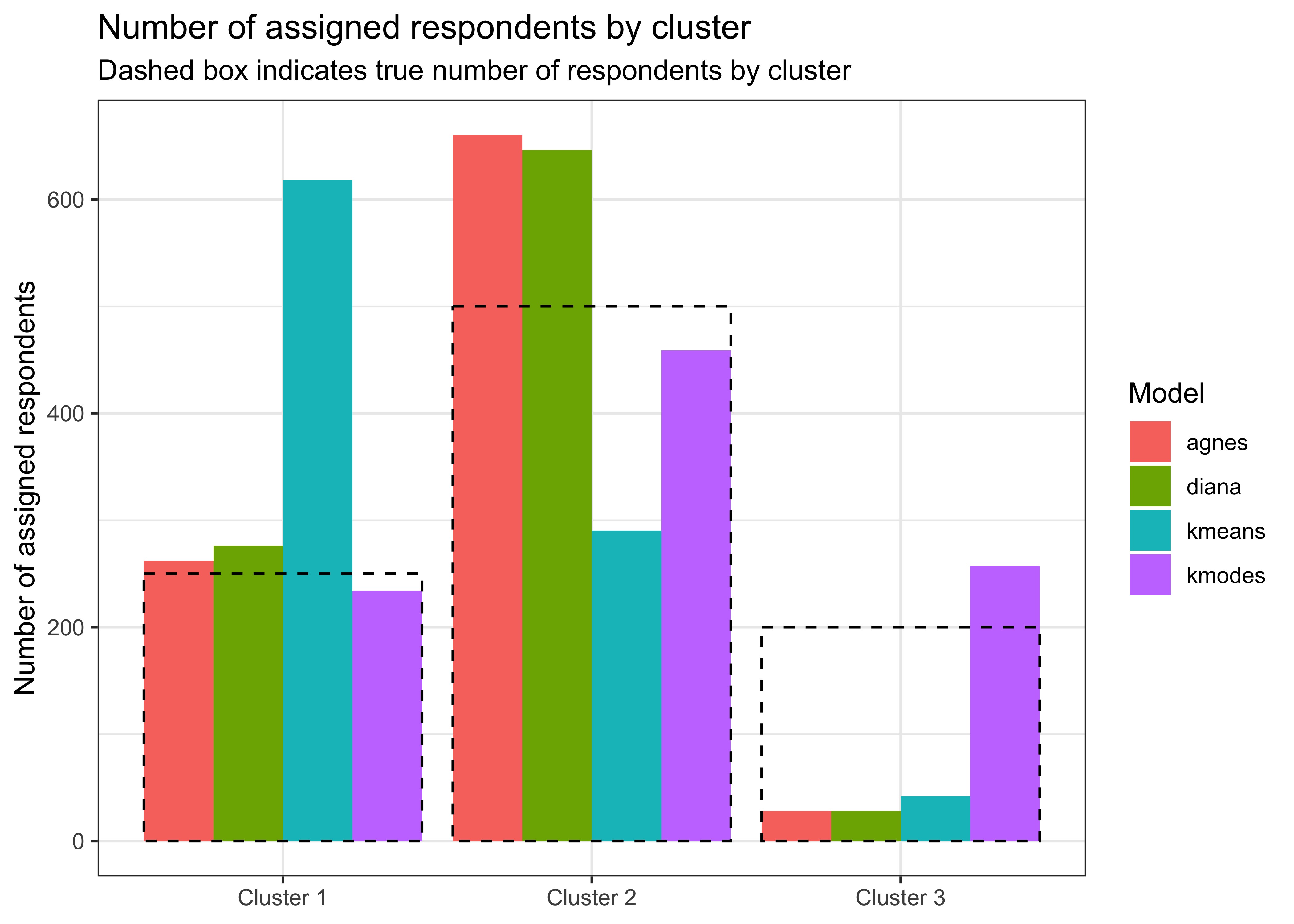
Let me end this post with a few words of caution: first, the ultimate outcome heavily depends on the seed chosen at the beginning of the post. The results might be quite different for other draws of respondents or initial conditions for clustering algorithms. Second, there are many more models out there that can be applied to the current setting. However, with this post I want to emphasize that it is important to consider different models at the same time and to compare them through a consistent set of measures. Ultimately, choosing the optimal number of clusters in practice requires a judgment call, but at least it can be informed as much as possible.
Footnotes
As of writing, the
tidyclustpackage only has limited support for hierarchical clustering, so I decided to abstain from using it for this post.↩︎