Tidy Fixed Effects Regressions: fixest vs pyfixest
A comparison of packages for fast fixed-effects estimation in R and Python
In this post, we’ll dive into how tidymodels can be leveraged to quickly prototype and compare classification models with tidy syntax. Classification models are a subset of machine learning models that are used to predict or classify the categories (aka classes) of new observations based on past observations with known category labels. Classification falls into the domain of supervised learning.
tidymodels is an ecosystem of R packages designed for data modeling and statistical analysis that adheres to the principles of the tidyverse. It provides a comprehensive framework for building and evaluating models, streamlining workflows from data pre-processing and feature engineering to model training, validation, and fine-tuning. As tidymodels provides a unified interface for various modeling techniques, it simplifies the process of creating reproducible and scalable data analysis pipelines, catering to both novice and experienced data scientists.
I’ll use the Telco Customer Churn data from IBM Sample Data Sets because it is a popular open-source data set used in predictive analytics, particularly for demonstrating the process of churn prediction. The data contains a mix of customer attributes, service usage patterns, and billing information, along with a churn indicator that specifies whether a customer has left the company.
We can download the telco customer churn data directly from the IBM GitHub account using the readr package. We immediately harmonize the column names using the janitor package. The raw data contains the following columns:
customer_id: A unique identifier for each customer.gender: The customer’s gender (male/female).senior_citizen: Indicates whether the customer is a senior citizen.partner: Indicates whether the customer has a partner.dependents: Indicates whether the customer has dependents.tenure: The number of months the customer has been with the company.phone_service: Indicates whether the customer has phone service.multiple_lines: Indicates whether the customer has multiple lines.internet_service: Type of internet service (DSL, Fiber optic, No).online_security: Indicates whether the customer has online security services.online_backup: Indicates whether the customer has online backup services.device_protection: Indicates whether the customer has device protection plans.tech_support: Indicates whether the customer has tech support services.streaming_tv: Indicates whether the customer has streaming TV services.streaming_movies: Indicates whether the customer has streaming movies services.contract: The contract term of the customer (Month-to-month, One year, Two year).paperless_billing: Indicates whether the customer has paperless billing.payment_method: The customer’s payment method (Electronic check, Mailed check, Bank transfer, Credit card).monthly_charges: The amount charged to the customer monthly.total_charges: The total amount charged to the customer.churn: Whether the customer churned or not (Yes or No).We start the data preparation by dropping all rows with missing values. We only use 11 observations, so there is no need to investigate or impute. We can also remove customer_id because we don’t need it for pre-processing. I make sure that all binary variables are encoded with binary indicators. We’ll apply one-hot encoding to the remaining variables later.
library(readr)
library(dplyr)
library(janitor)

data_url <- "https://raw.githubusercontent.com/IBM/telco-customer-churn-on-icp4d/master/data/Telco-Customer-Churn.csv"
customer_raw <- read_csv(data_url) |>
  clean_names()

customer <- customer_raw |>
  select(-customer_id) |>
  na.omit() |>
  mutate(churn = factor(if_else(churn=="Yes", 1L, 0L)),
         female = if_else(gender=="Female", 1L, 0L),
         senior_citizen = as.integer(senior_citizen)) |>
  select(-gender) |>
  mutate(
    across(c(partner, dependents, phone_service, paperless_billing),
           ~if_else(. == "Yes", 1L, 0L)),
    across(c(multiple_lines, internet_service, online_security, online_backup,
             device_protection, tech_support, streaming_tv, streaming_movies,
             contract, paperless_billing, payment_method),
           ~tolower(gsub("[ |\\-]", "_", ., " |\\-", "_")))
    )
We next prepare the data for machine learning model training and evaluation by creating a reproducible initial split into training and test sets, followed by setting up a stratified 5-fold cross-validation scheme on the training data. This approach is crucial for developing, tuning, and selecting models based on their performance metrics, ensuring that the chosen model is robust and performs well on unseen data.
library(tidymodels)

set.seed(1234)
customer_split <- initial_split(customer, prop = 4/ 5, strata = churn)
customer_folds <- vfold_cv(training(customer_split), v = 5, strata = churn)Data pre-processing is implemented via recipe() in the tidymodels framework. A recipe defines a series of data pre-processing steps to prepare the training data for modeling. I chose to transforme total_charges (to handle its skewed distribution), normalize tenure and monthly_charges, and encode categorical variables as dummy variables. one_hot = TRUE specifies that one-hot encoding should be used, where each level of the categorical variables is transformed into a new binary column, with a value of 1 if the observation belongs to that level and 0 otherwise. This is necessary because many machine learning models cannot directly handle categorical variables and require them to be converted into a numeric format.
customer_recipe <- recipe(churn ~ ., data = training(customer_split)) |>
  step_log(c(total_charges)) |>
  step_normalize(c(tenure, monthly_charges)) |>
  step_dummy(all_nominal(), -all_outcomes(), one_hot = TRUE)
This pre-processing is crucial for ensuring that the data is in the right format and scale for the algorithms to work effectively, ultimately leading to more accurate and reliable model predictions.
A workflow() in the tidymodels framework encapsulates all the components needed to train a machine learning model, including pre-processing instructions (via recipes) and the model itself. So, we start by initializing our workflow with the recipe and add other components later.
customer_workflow <- workflow() |>
add_recipe(customer_recipe)Logistic Regression is a statistical method for predicting binary outcomes. The outcome is modeled as a function of predictor variables using the logistic function to ensure that the predictions fall between 0 and 1, which are then interpreted as probabilities of belonging to a particular class.
glmnet is an R package that fits generalized linear models via penalized maximum likelihood. The penalty term is a combination of the L1 norm (lasso) and the L2 norm (ridge) of the coefficients. If you want to learn more about this model, check out our chapter on Factor Selection via Machine Learning in Tidy Finance with R.
By specifying a logistic regression model with a slight L1 penalty (lasso) using the glmnet engine, we’re aiming to build a model that can predict binary outcomes, while also performing feature selection to keep the model simple and prevent overfitting.
library(glmnet)

spec_logistic <- logistic_reg(penalty = 0.0001, mixture = 1) |>
  set_engine("glmnet") |>
  set_mode("classification")
At its core, a Random Forest model consists of many decision trees. A decision tree is a simple model that makes decisions based on answering a series of questions based on the features of the data. The ranger package provides a fast and efficient implementation of Random Forests and is able to handle large data sets and high-dimensional data well.
library(ranger)

spec_random_forest <- rand_forest() |>
  set_engine("ranger") |>
  set_mode("classification")
XGBoost stands for eXtreme Gradient Boosting. It is part of a family of boosting algorithms which are based on the principle of gradient boosting. Boosting, in the context of machine learning, refers to the technique of sequentially building models, where each new model attempts to correct the errors of the previous ensemble of models. Unlike Random Forests, where each tree is built independently, XGBoost builds one tree at a time. Each new tree in XGBoost learns from the mistakes of the previous trees.
library(xgboost)

spec_xgboost <- boost_tree() |>
  set_engine("xgboost") |>
  set_mode("classification")
The k-Nearest Neighbors algorithm operates on a very simple principle: “Tell me who your neighbors are, and I will tell you who you are.” For a given data point that we wish to classify, the algorithm looks at the ‘k’ closest points (neighbors) to it in the data, based on a distance metric (typically Euclidean distance). The class that is most common among these neighbors is then assigned to the data point.
library(kknn)

spec_knn <- nearest_neighbor(neighbors = 4) |>
  set_engine("kknn") |>
  set_mode("classification")
Intuitively, neural networks try to mimic the way human brains operate, albeit in a very simplified form. A neural network consists of layers of interconnected nodes (neurons), where each connection (synapse) carries a weight that signifies the importance of the input it’s receiving. The basic idea is that, through a process of learning, the network adjusts these weights to make accurate predictions or classifications.
A mulit-layer-perceptron (MLP) is a type of neural network that includes one or more hidden layers between the input and output layers. Each layer’s output is passed through an activation function, which allows the network to capture complex patterns in the data. hidden_units = 10 specifies that there are 10 neurons in a single hidden layer and epochs = 500 indicates the number of times the learning algorithm will work through the entire training data.
library(torch)
library(brulee)

spec_neural_net <- mlp(epochs = 500, hidden_units = 10) |>
  set_engine("brulee") |>
set_mode("classification") Now that we have defined a couple of models, we want to fit them to the training data next. As stated above, we use cross-validation and we look at multiple metrics (recall, precision, and accuracy). Since the approach is the same across model specifications, I wrote a little helper function that adds the model to the workflow, fits the model using the customer_folds from above, and collects the metrics of interest. We can then simply map this function across specifications and get a table of metrics.
create_metrics_training <- function(spec) {
  customer_workflow |>
    add_model(spec) |>
    fit_resamples(
      resamples = customer_folds,
      metrics = metric_set(recall, precision, accuracy),
      control = control_resamples(save_pred = TRUE)
    ) |>
    collect_metrics(summarize = TRUE) |>
    mutate(model = attributes(spec)$class[1])
}

metrics_training <- list(
  spec_logistic, spec_random_forest, spec_xgboost,
  spec_knn, spec_neural_net
) |>
map_df(create_metrics_training)The first step in model evaluation is to compare the metrics of interest based on training data. We focus on the average for each metric and model across the different folds. However, I also add confidence intervals to the metrics to illustrate the dispersion across folds.
We can see that the nearest neighbor approach shows the worst performance across all metrics, while the other exhibit very similar performance. The logistic regression and neural network seem to be in the lead, but there is no clear winner because their confidence intervals overlap.
metrics_training |>
  mutate(ci_lower = mean - std_err / sqrt(n) * qnorm(0.99),
         ci_upper = mean + std_err / sqrt(n) * qnorm(0.99)) |>
  ggplot(aes(x = mean, y = model, fill = model)) +
  geom_col() +
  geom_errorbar(aes(xmin = ci_lower, xmax = ci_upper), width = .2,
                position = position_dodge(.9)) +
  facet_wrap(~.metric, ncol = 1) +
  labs(x = NULL, y = NULL,
       title = "Comparison of metrics for different classification models",
       subtitle = "Based on training data. Error bars indicate 99% confidence intervals.") +
  theme_minimal() +
  theme(legend.position = "none") +
coord_cartesian(xlim = c(0, 1)) 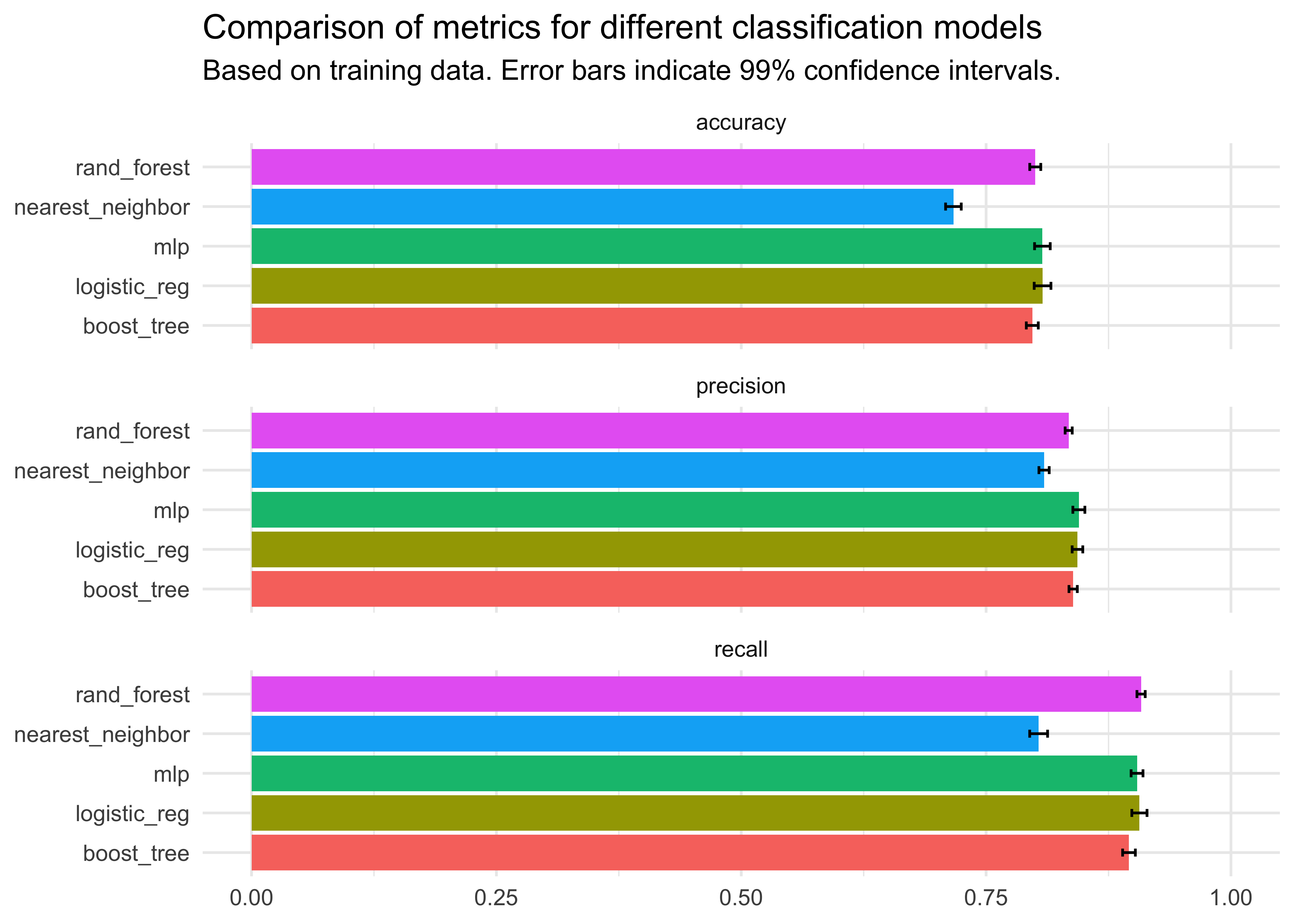
The second important evaluation step involves fitting the models to the training data and then using the fitted models to create predictions in the test sample. Again, I created a helper function that can be mapped across different model specifications.
create_metrics_test <- function(spec) {

  test_predictions <-  customer_workflow |>
    add_model(spec) |>
    fit(data =  training(customer_split)) |>
    predict(new_data = testing(customer_split))

  test_results <- bind_cols(testing(customer_split), test_predictions)

  bind_rows(
    recall(test_results, truth = churn, estimate = .pred_class),
    precision(test_results, truth = churn, estimate = .pred_class),
    accuracy(test_results, truth = churn, estimate = .pred_class)
  ) |>
    mutate(model = attributes(spec)$class[1])
}

metrics_test <- list(
  spec_logistic, spec_random_forest, spec_xgboost,
  spec_knn, spec_neural_net
) |>
  map_df(create_metrics_test)
Let’s compare the performance of models in the training to the test sample. We can see that the models perform similarly across samples, which is good.
metrics <- bind_rows(
  metrics_training |>
    mutate(sample = "Training") |>
    select(metric = .metric, estimate = mean, model, sample),
  metrics_test |>
    mutate(sample = "Test") |>
    select(metric = .metric, estimate = .estimate, model, sample)
)

metrics |>
  ggplot(aes(x = estimate, y = model, fill = sample)) +
  geom_col(position = "dodge") +
  facet_wrap(~metric, ncol = 1) +
  labs(x = NULL, y = NULL, fill = "Sample",
       title = "Comparison of metrics for different classification models",
       subtitle = paste0("Training is the mean across 5-fold cross validation results.\n",
                         "Test is based on 20% of the initial data.")) +
  theme_minimal() +
coord_cartesian(xlim = c(0, 1)) 
To fit the models above, we simply imposed a couple of values for the hyperparameters of each model. I recommend you to check out the tidymodels documentation to learn more about the defaults that it implements in its functions. Model tuning is the process of optimally selecting such hyperparameters. tidymodels provides extensive tuning options based on cross-validation.
The general idea is to create a grid of parameter values that you want to tune and then fit the model to the training data using cross-validation for each parameter combination. This step is typically computationally quite expensive because it involves a lot of estimations. So in practice, you’d typically choose the best model from the previous evaluation step and tune it. The code chunks below show you how to tune each model and the resulting best model. However, note that I only pick 2 hyperparameters to tune for each model although most models have more paraters.
spec_logistic_tune <- logistic_reg(
  penalty = tune(),
  mixture = tune()
) |>
  set_engine("glmnet") |>
  set_mode("classification")

grid_logistic <- grid_regular(
  penalty(range = c(-10, 0), trans = log10_trans()),
  mixture(range = c(0, 1)),
  levels = 5
)

tune_logistic <- tune_grid(
  customer_workflow |>
    add_model(spec_logistic_tune),
  resamples = customer_folds,
  grid = grid_logistic,
  metrics = metric_set(recall, precision, accuracy)
)

tuned_model_logistic <- finalize_model(
  spec_logistic_tune, select_best(tune_logistic, "accuracy")
)
tuned_model_logistic
Logistic Regression Model Specification (classification)
Main Arguments:
penalty = 1e-10
mixture = 0
Computational engine: glmnet spec_random_forest_tune <- rand_forest(
mtry = tune(),
min_n = tune()
) |>
set_engine("ranger") |>
set_mode("classification")
grid_random_forest <- grid_regular(
mtry(range = c(1, 5)),
min_n(range = c(2, 40)),
levels = 5
)
tune_random_forest <- tune_grid(
customer_workflow |>
add_model(spec_random_forest_tune),
resamples = customer_folds,
grid = grid_random_forest,
metrics = metric_set(recall, precision, accuracy)
)
tuned_model_random_forest <- finalize_model(
spec_random_forest_tune, select_best(tune_random_forest, "accuracy")
)
tuned_model_random_forestRandom Forest Model Specification (classification)
Main Arguments:
mtry = 5
min_n = 40
Computational engine: ranger spec_xgboost_tune <- boost_tree(
mtry = tune(),
min_n = tune()
) |>
set_engine("xgboost") |>
set_mode("classification")
grid_xgboost <- grid_regular(
mtry(range = c(1L, 5L)),
min_n(range = c(1L, 40L)),
levels = 5
)
tune_xgboost <- tune_grid(
customer_workflow |>
add_model(spec_xgboost_tune),
resamples = customer_folds,
grid = grid_xgboost,
metrics = metric_set(recall, precision, accuracy)
)
tuned_model_xgboost <- finalize_model(
spec_xgboost_tune, select_best(tune_xgboost, "accuracy")
)
tuned_model_xgboostBoosted Tree Model Specification (classification)
Main Arguments:
mtry = 5
min_n = 40
Computational engine: xgboost grid_knn <- grid_regular(
neighbors(range = c(1L, 20L)),
levels = 5
)
spec_knn_tune <- nearest_neighbor(
neighbors = tune()
) |>
set_engine("kknn") |>
set_mode("classification")
tune_knn <- tune_grid(
customer_workflow |>
add_model(spec_knn_tune),
resamples = customer_folds,
grid = grid_knn,
metrics = metric_set(recall, precision, accuracy)
)
tuned_model_knn <- finalize_model(spec_knn_tune, select_best(tune_knn, "accuracy"))
tuned_model_knnK-Nearest Neighbor Model Specification (classification)
Main Arguments:
neighbors = 20
Computational engine: kknn grid_neural_net <- grid_regular(
hidden_units(range = c(1L, 10L)),
epochs(range = c(10L, 1000L)),
levels = 5
)
spec_neural_net_tune <- mlp(
epochs = tune(),
hidden_units = tune()
) |>
set_engine("brulee") |>
set_mode("classification")
tune_neural_net <- tune_grid(
customer_workflow |>
add_model(spec_neural_net_tune),
resamples = customer_folds,
grid = grid_neural_net,
metrics = metric_set(recall, precision, accuracy)
)
tuned_model_neural_net <- finalize_model(spec_neural_net_tune, select_best(tune_neural_net, "accuracy"))
tuned_model_neural_netSingle Layer Neural Network Model Specification (classification)
Main Arguments:
hidden_units = 10
epochs = 1000
Computational engine: brulee Now, that we have used tuning to find better models than our initial guesses, we can again compare the model performance in different samples.
metrics_tuned <- list(
  tuned_model_logistic, tuned_model_random_forest, tuned_model_xgboost,
  tuned_model_knn, tuned_model_neural_net
) |>
  map_df(create_metrics_test)

metrics_comparison <- bind_rows(
  metrics,
  metrics_tuned |>
    mutate(sample = "Tuned") |>
    select(metric = .metric, estimate = .estimate, model, sample)
)
I only plot the accuracy measure below to avoid visual overload. We can see that the fine tuning significantly improved the performance of the nearest neighbor algorithm, but it had little impact on the other approaches. One explanation for the lack of dramatic increases in model performance might be that I picked the wrong parameters for tuning, so I encourage you to play around with the hyperparameters.
metrics_comparison |>
  filter(metric == "accuracy") |>
  ggplot(aes(x = estimate, y = model, fill = sample)) +
  geom_col(position = "dodge") +
  facet_wrap(~metric, ncol = 1) +
  labs(x = NULL, y = NULL, fill = "Sample",
       title = "Comparison of accuracy for different classification models",
       subtitle = paste0("Training is the mean across 5-fold cross validation results of inital models.\n",
                         "Test is based on 20% of the initial data using the initial models.\n",
                         "Tuned is based on 20% of the initial data using the fine-tuned models.")) +
  theme_minimal() +
coord_cartesian(xlim = c(0, 1)) 
So what is the best model now for the classification problem? There are so many different measures and ways to evaluate models that it might be hard to draw conclusions. I usually go with the following heuristic: which model has on average the best rank across all measures and samples? It turns out that the logistic regression is most often on top, followed by the neural network. This finding is interesting because the logistic regression is quite simple and computationally relatively inexpensive. A natural next step would be to extend the neural network to multiple layers and find a deep neural net that is able to consistently beat the logistic regression.
metrics_comparison |>
  group_by(sample, metric) |>
  arrange(-estimate) |>
  mutate(rank = row_number()) |>
  group_by(model) |>
  summarize(rank = mean(rank)) |>
  arrange(rank)
# A tibble: 5 × 2
model rank
<chr> <dbl>
1 mlp 1.89
2 logistic_reg 2.11
3 rand_forest 2.11
4 boost_tree 3.89
5 nearest_neighbor 5 Overall, this blog post illustrates what I love most about tidymodels: its scalability with respect to models and metrics. You can quickly prototype different approaches using very little code.
Is your favorite algorithm missing? Let me know in the comments below, and I’ll try to incorporate it in this blog post using tidymodels.